Testing Radial
Testing spatial frequency component
In [1]:
import numpy as np
np.set_printoptions(precision=5, suppress=True)
import pylab
import matplotlib.pyplot as plt
%matplotlib inline
#!rm -fr ../files/radial*
In [2]:
import MotionClouds as mc
import os
fx, fy, ft = mc.get_grids(mc.N_X, mc.N_Y, mc.N_frame)
help(mc.envelope_radial)
In [3]:
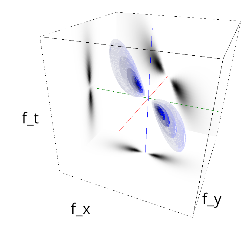
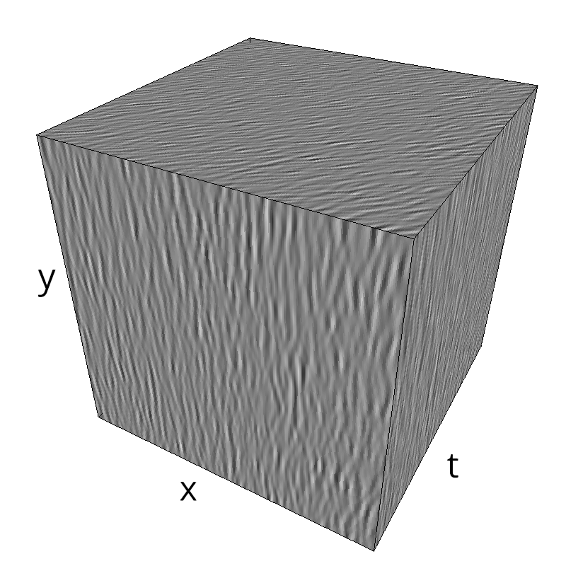
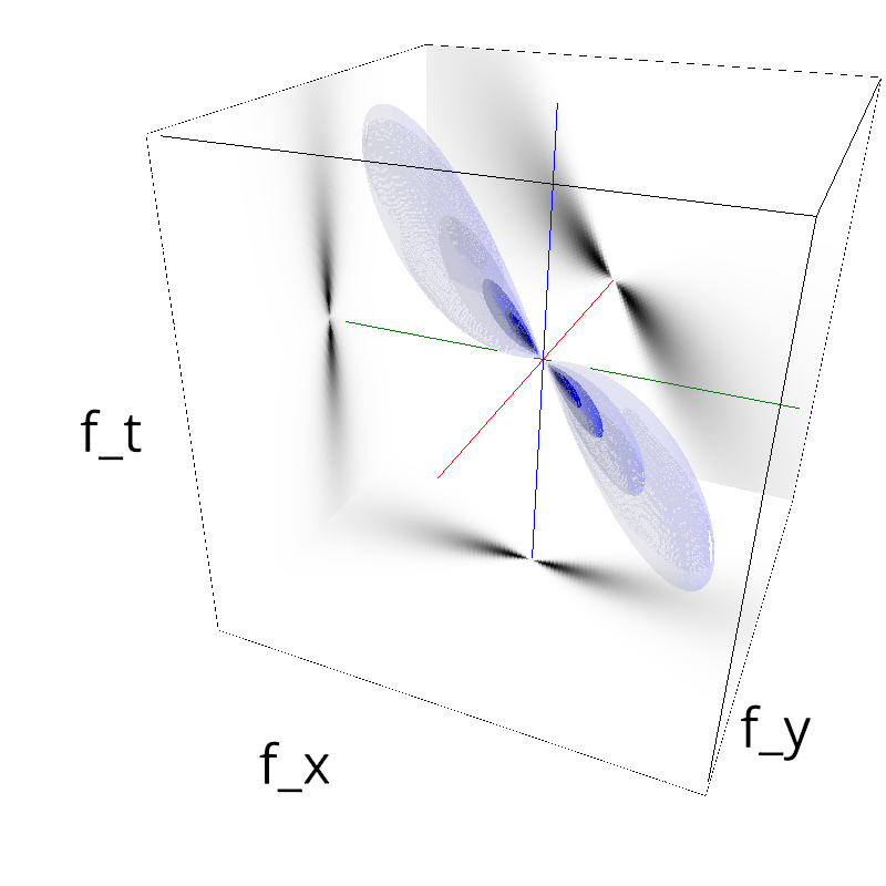
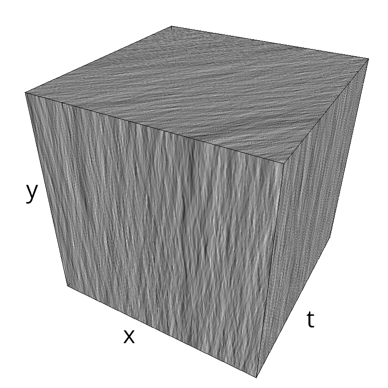
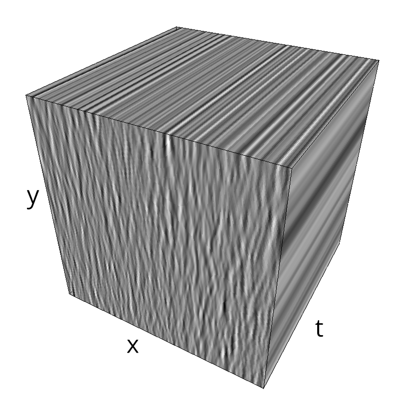
name = 'radial'
#initialize
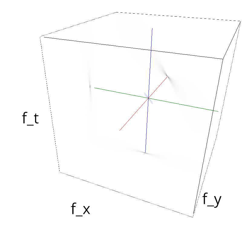
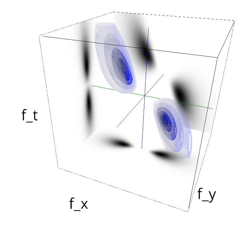
fx, fy, ft = mc.get_grids(mc.N_X, mc.N_Y, mc.N_frame)
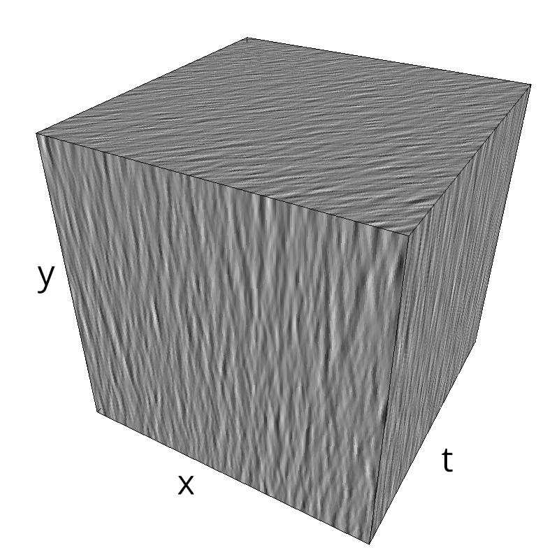
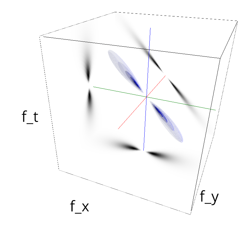
mc.figures_MC(fx, fy, ft, name)
verbose = False
mc.in_show_video(name)
 |
||
 |
||
In [4]:
N = 5
np.logspace(-5, 0., 7, base=2)
Out[4]:
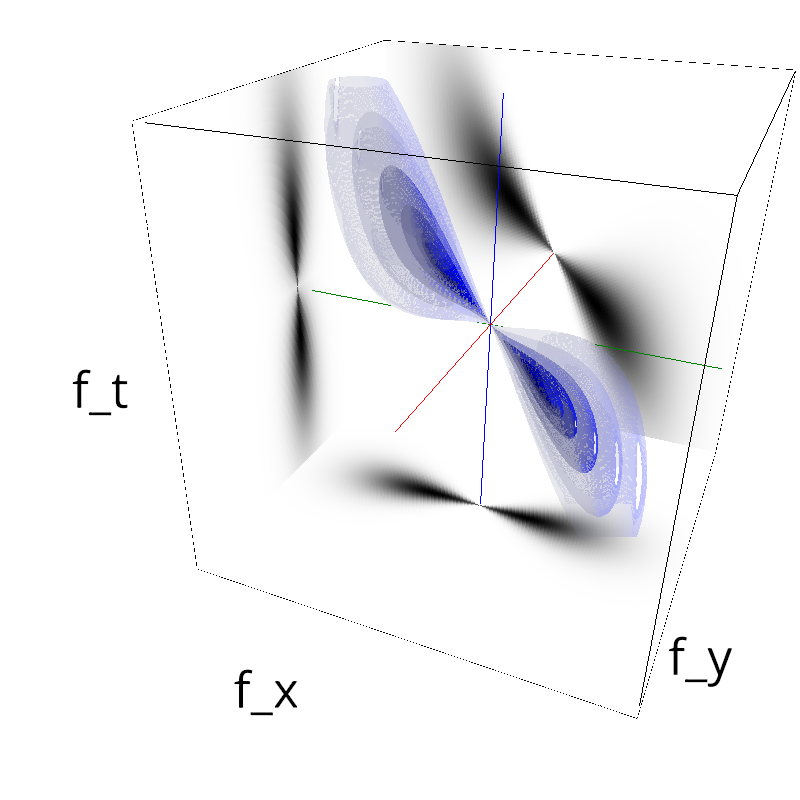
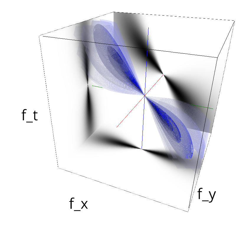
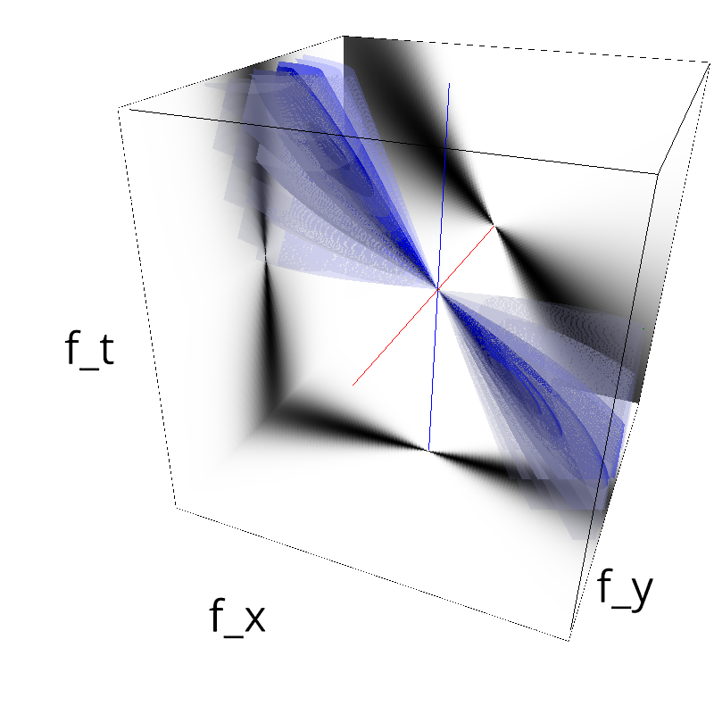
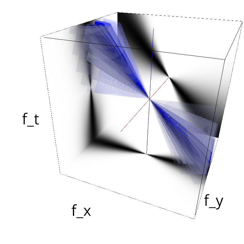
exploring different frequency bandwidths
In [5]:
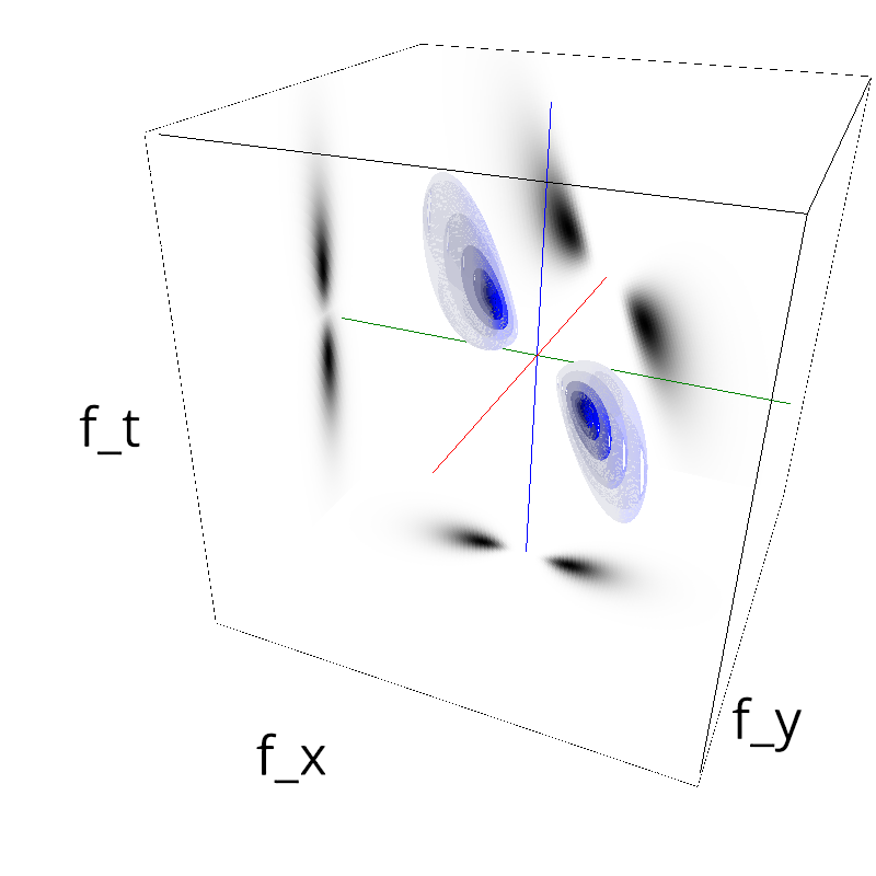
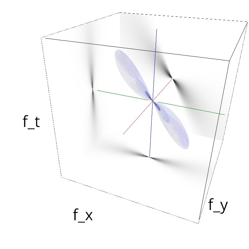
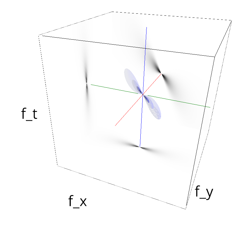
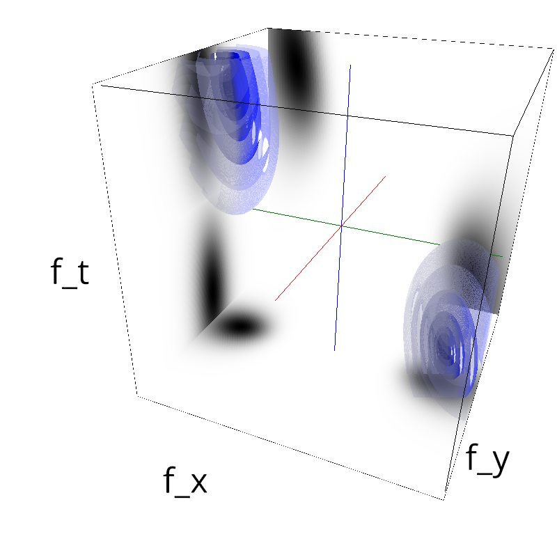
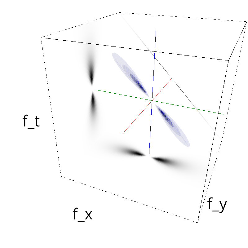
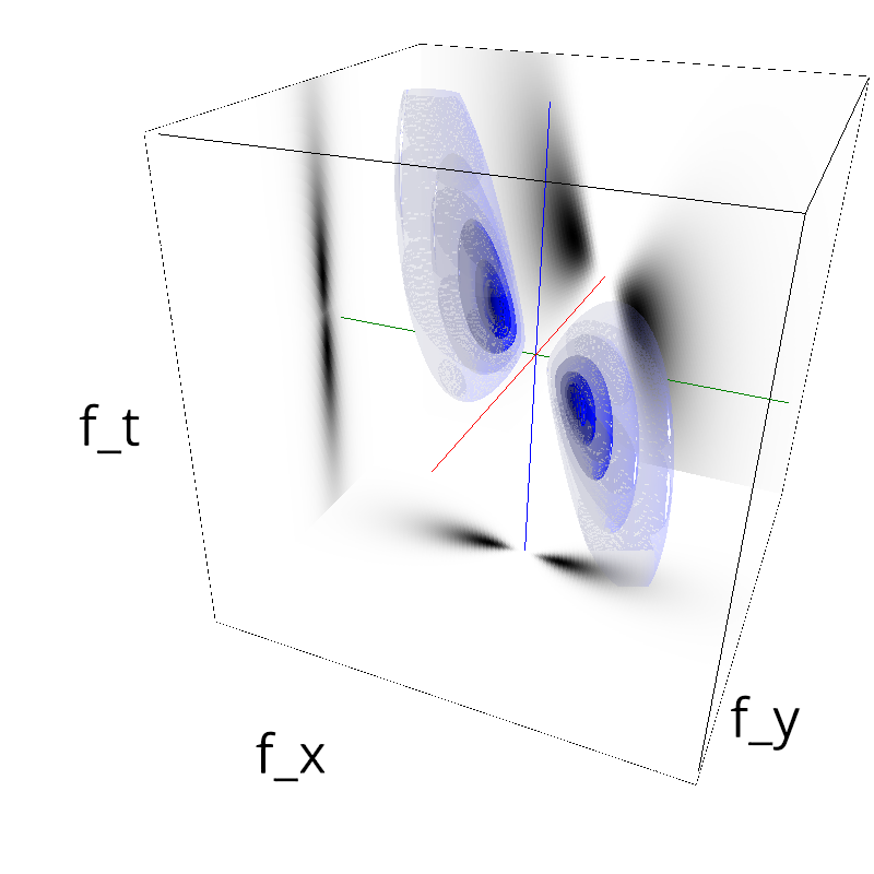
for B_sf in np.logspace(-4, 0., N, base=2):
    name_ = name + '-B_sf-' + str(B_sf).replace('.', '_')
    mc.figures_MC(fx, fy, ft, name_, B_sf=B_sf, verbose=verbose)
    mc.in_show_video(name_)
 |
||
 |
||
 |
||
 |
||
 |
||
 |
||
 |
||
 |
||
 |
||
 |
||
exploring different (median) central frequencies
In [6]:
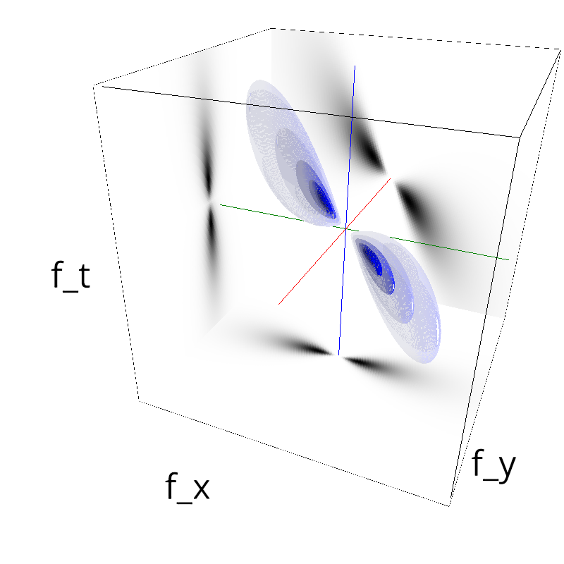
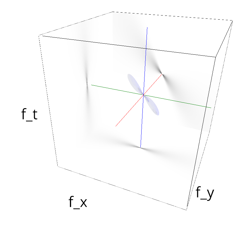
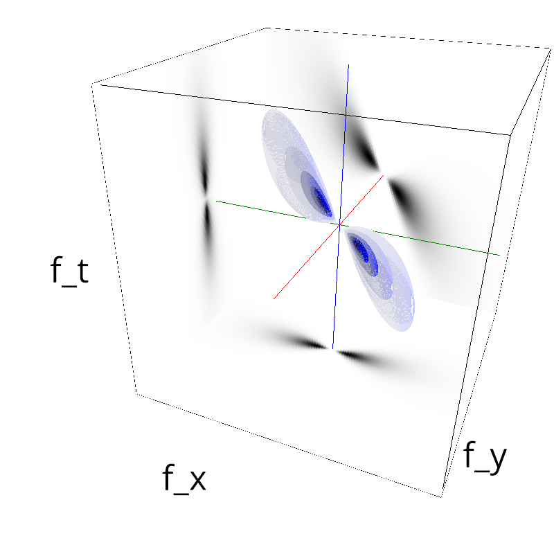
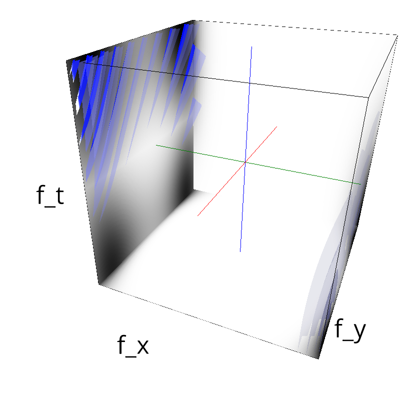
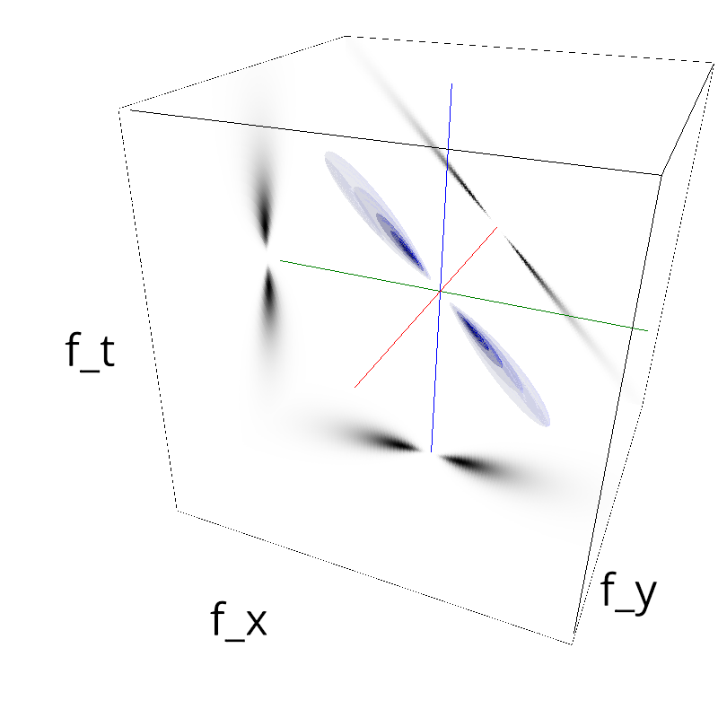
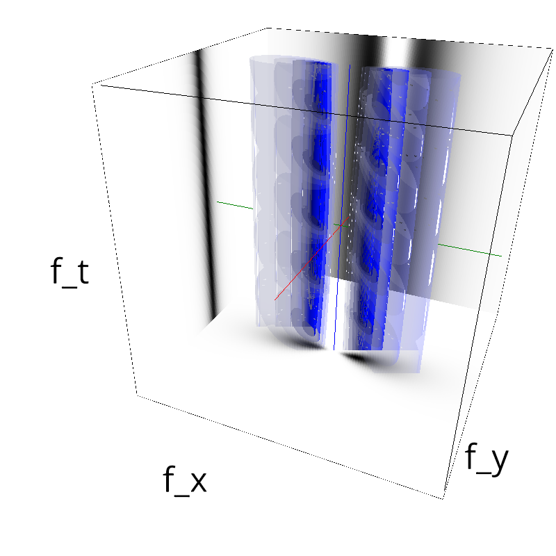
for sf_0 in [0.01, 0.05, 0.1, 0.2, 0.4, 0.8]:
    name_ = name + '-sf_0-' + str(sf_0).replace('.', '_')
    mc.figures_MC(fx, fy, ft, name_, sf_0=sf_0, verbose=verbose)
    mc.in_show_video(name_)
 |
||
 |
||
 |
||
 |
||
 |
||
 |
||
 |
||
 |
||
 |
||
 |
||
 |
||
 |
||
Note that some information is lost in the last case as $f_0$ exceeds the Nyquist frequency.
exploring different speed bandwidths
In [7]:
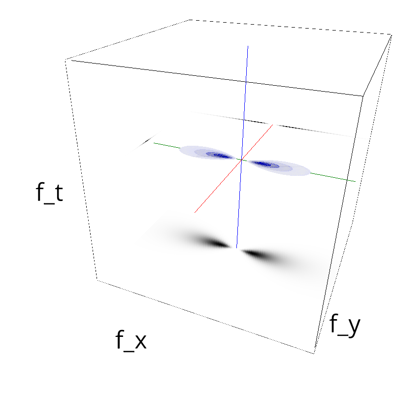
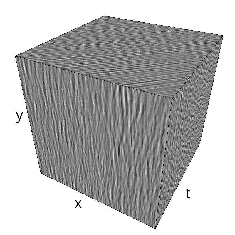
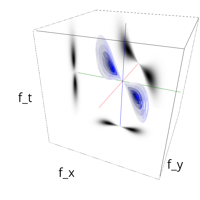
for B_V in [0, 0.001, 0.01, 0.05, 0.1, 0.5, 1.0, 10.0]:
    name_ = name + '-B_V-' + str(B_V).replace('.', '_')
    mc.figures_MC(fx, fy, ft, name_, B_V=B_V, verbose=verbose)
    mc.in_show_video(name_)
 |
||
 |
||
 |
||
 |
||
 |
||
 |
||
 |
||
 |
||
 |
||
 |
||
 |
||
 |
||
 |
||
 |
||
 |
||
 |
||
Testing without using a log-normal distribution
In [8]:
for B_sf in np.logspace(-4, 0., N, base=2):
    name_ = name + '-B_sf_nologgabor-' + str(B_sf).replace('.', '_')
    mc.figures_MC(fx, fy, ft, name_, B_sf=B_sf, loggabor=False, verbose=verbose)
    mc.in_show_video(name_)
 |
||
 |
||
 |
||
 |
||
 |
||
 |
||
 |
||
 |
||
 |
||
 |
||
checking that sf_0 is consistant with the number of cycles per period
By design, MotionClouds are created to be characterized by a given frequency range. Let's check on the raw image that this is correct.
In [9]:
downscale = 4
fx, fy, ft = mc.get_grids(mc.N_X/downscale, mc.N_Y/downscale, mc.N_frame/downscale)
N_X, N_Y, N_frame = fx.shape

def spatial_xcorr(im):
    import scipy.ndimage as nd
    N_X, N_Y, N_frame = im.shape
    Xcorr = np.zeros((N_X, N_Y))
    for t in range(N_frame):
        Xcorr += nd.correlate(im[:, :, t], im[:, :, t], mode='wrap')
    return Xcorr

mc_i = mc.envelope_gabor(fx, fy, ft,
                         V_X=0., V_Y=0.,
                         sf_0=0.15, B_sf=0.03)
im = mc.random_cloud(mc_i)
Xcorr = spatial_xcorr(im)
plt.imshow(Xcorr)
Out[9]:

In [10]:
xcorr = Xcorr.sum(axis=1)
xcorr /= xcorr.max()
plt.plot(np.arange(-N_X/2, N_X/2), xcorr)
print('First maximum reached at index ' + str(np.argmax(xcorr)) + ' - that is normal as we plot the autocorrelation')
print('Max = ', xcorr[np.argmax(xcorr)])

To find the period, intuitively, one could just find the zero of the gradient:
In [11]:
half_xcorr = xcorr[N_X//2:]
half_xcorr_gradient = np.gradient(xcorr)[N_X//2:]
plt.plot(half_xcorr)
plt.plot(half_xcorr_gradient, 'g')
idx = np.argmax(half_xcorr_gradient>0)
print('First zero gradient reached at index ' + str(idx) + ' - at the minimum of the xcorr')
print (half_xcorr_gradient[idx-1], half_xcorr_gradient[idx])

We thus get in pixels half of the width of a period.
More precisely, let's fit with a sinusoid (that's yet another FFT...):
In [12]:
xcorr_MC = np.absolute(mc_i**2).sum(axis=-1).sum(axis=-1)
half_xcorr_MC = xcorr_MC[N_X//2:]
half_xcorr_MC /= half_xcorr_MC.max()
plt.plot(half_xcorr_MC, 'r--')

half_xcorr_FT = np.absolute(np.fft.fft(xcorr))[:N_X//2]
half_xcorr_FT /= half_xcorr_FT.max()
plt.plot(half_xcorr_FT)
idx = np.argmax(half_xcorr_FT)
print('Max auto correlation reached at frequency ' + str(idx))
print('Max auto correlation reached with a period ' + str(1.*N_X/idx))

Wrapping things up:
In [13]:
sf_0_ = [0.01, 0.05, 0.1, 0.2, 0.4, 0.8]
sf_0_ = np.linspace(0.01, .5, 12)
downscale = 4
fx, fy, ft = mc.get_grids(mc.N_X//downscale, mc.N_Y//downscale, mc.N_frame//downscale)

def period_px(mc_i):
    N_X, N_Y, N_frame = im.shape
    xcorr_MC = np.absolute(mc_i**2).sum(axis=-1).sum(axis=-1)
    half_xcorr_MC = xcorr_MC[N_X//2:]
    idx = np.argmax(half_xcorr_MC)
    return np.fft.fftfreq(N_X)[idx]

ppx = np.zeros_like(sf_0_)
for i, sf_0 in enumerate(sf_0_):
    mc_i = mc.envelope_gabor(fx, fy, ft,
                             V_X=0., V_Y=0.,
                             sf_0=sf_0, B_sf=0.03)
    ppx[i] = period_px(mc_i)

plt.plot(sf_0_, ppx)
plt.xlabel('sf_0 [a. u.]')
plt.ylabel('observed freq [a. u.]')
Out[13]:

Note that the range of frequencies is accessible using:
In [14]:
print(np.fft.fftfreq(fx.shape[0]))