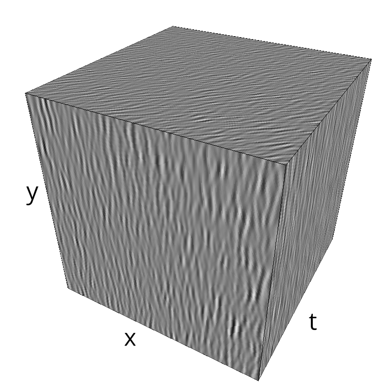
Testing Grating
testing the orientation component
On this page, we concerntrate on the orientation variable and test the effect of changing the average orientation as well as the bandwidth.
import numpy as np
np.set_printoptions(precision=3, suppress=True)
import pylab
import matplotlib.pyplot as plt
%matplotlib inline
%load_ext autoreload
%autoreload 2
import MotionClouds as mc
import os
fx, fy, ft = mc.get_grids(mc.N_X, mc.N_Y, mc.N_frame)
help(mc.envelope_orientation)
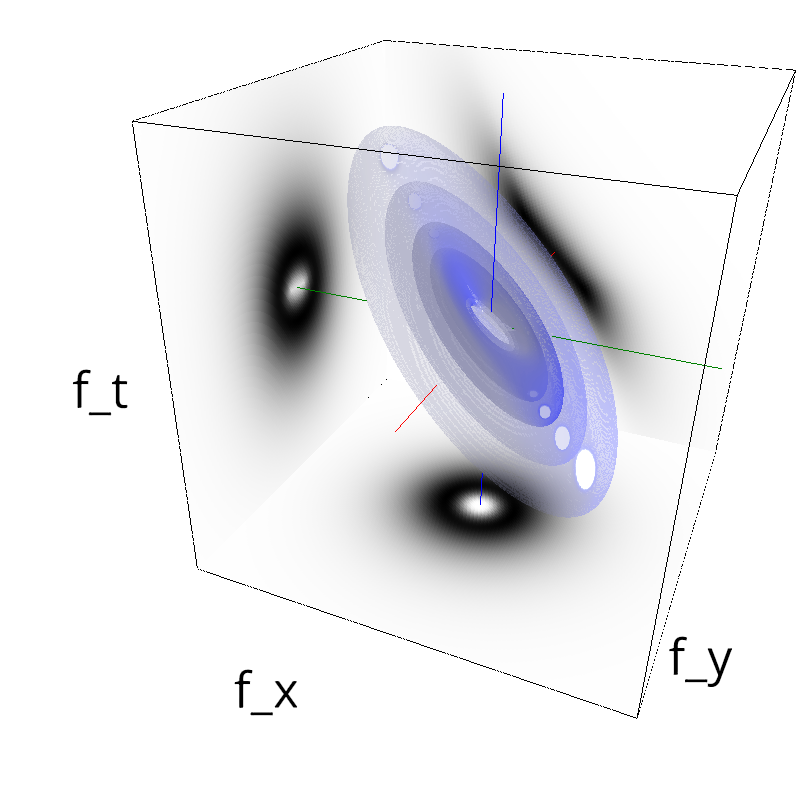
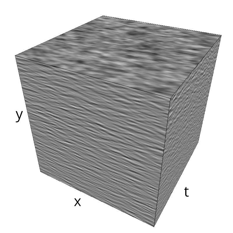
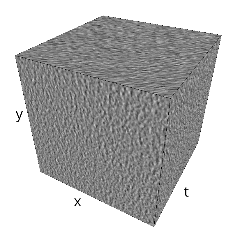
name = 'grating'
#initialize
fx, fy, ft = mc.get_grids(mc.N_X, mc.N_Y, mc.N_frame)

z = mc.envelope_gabor(fx, fy, ft)
mc.figures(z, name, vext='.gif')
mc.figures(z, name)
mc.in_show_video(name)
 |
||
 |
||
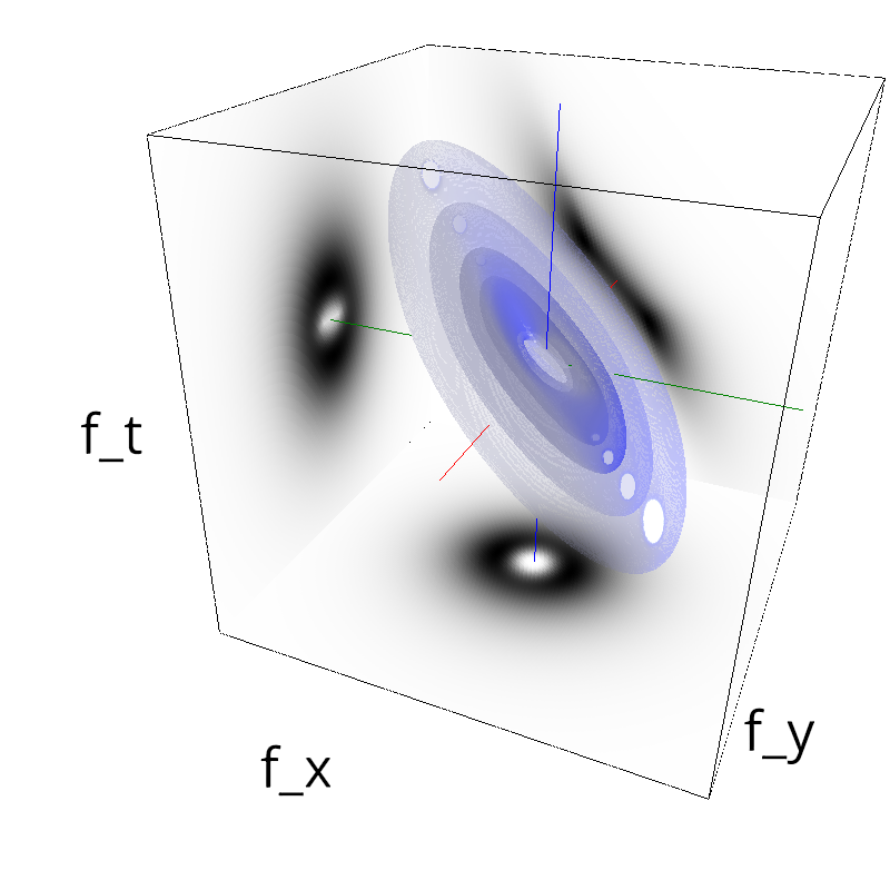
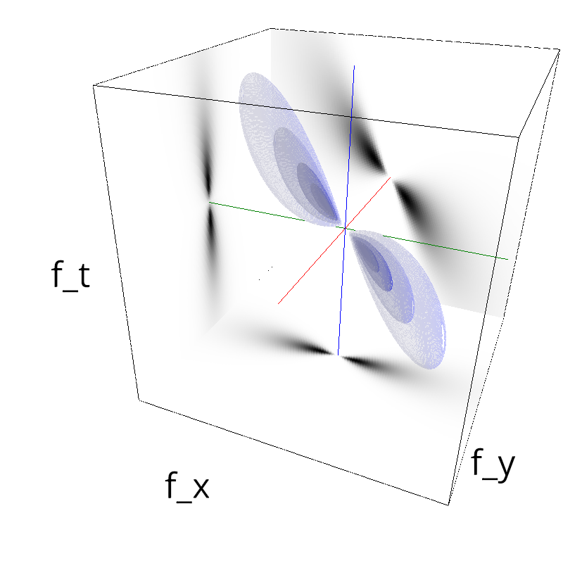
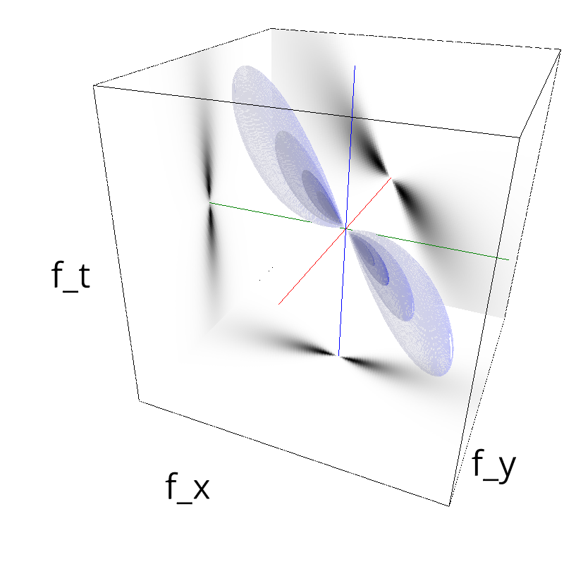
# explore parameters
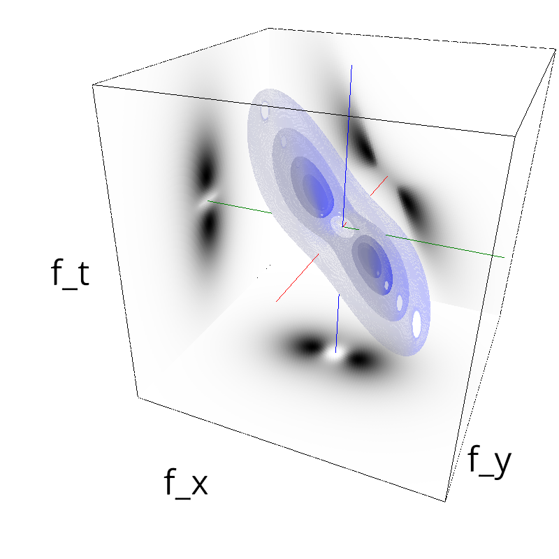
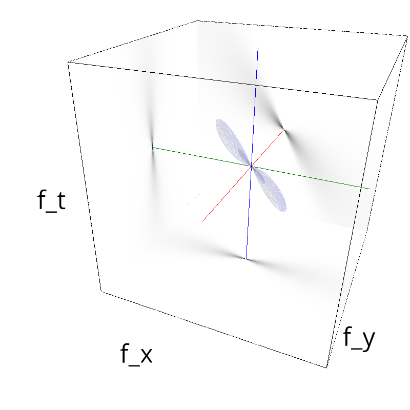
for sigma_div in [1, 2, 3, 5, 8, 13 ]:
name_ = name + '-largeband-B_theta-pi-over-' + str(sigma_div).replace('.', '_')
z = mc.envelope_gabor(fx, fy, ft, B_theta=np.pi/sigma_div)
mc.figures(z, name_)
mc.in_show_video(name_)
 |
||
 |
||
 |
||
 |
||
 |
||
 |
||
 |
||
 |
||
 |
||
 |
||
 |
||
 |
||
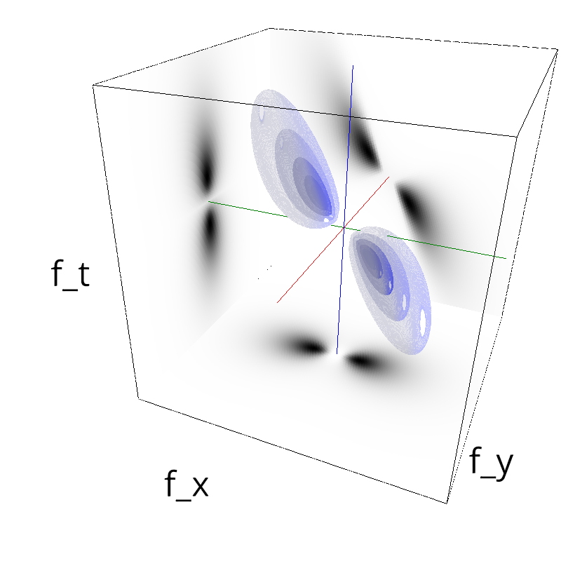
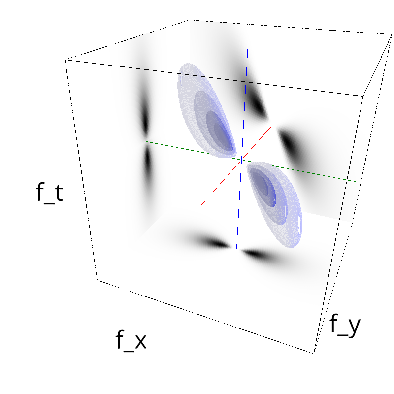
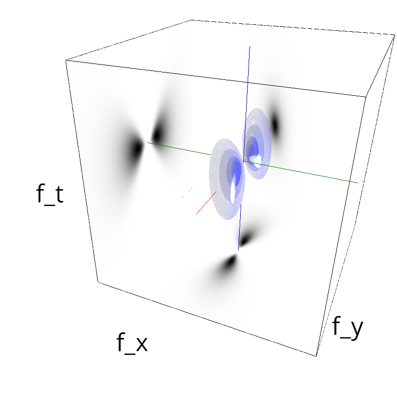
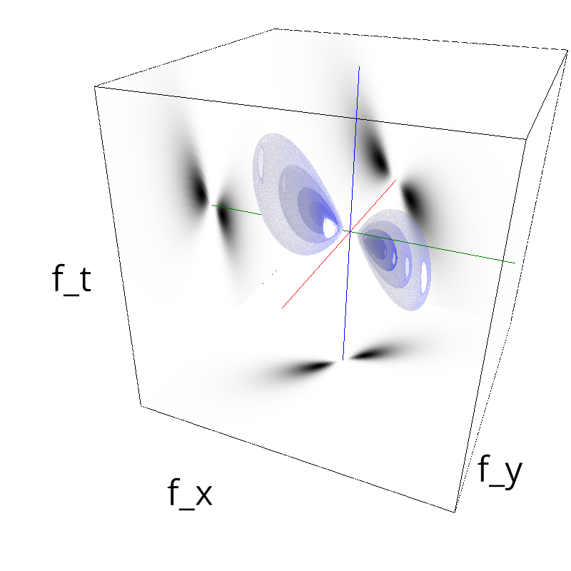
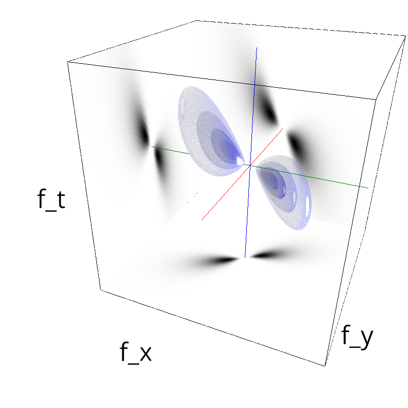
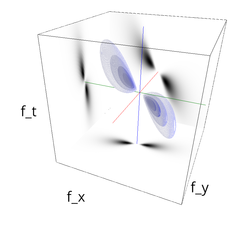
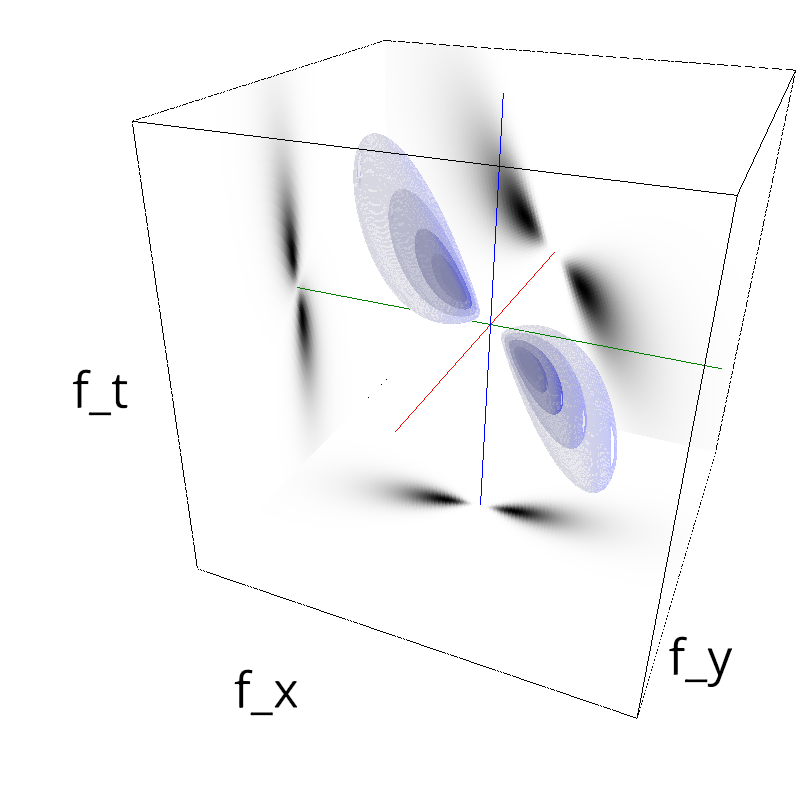
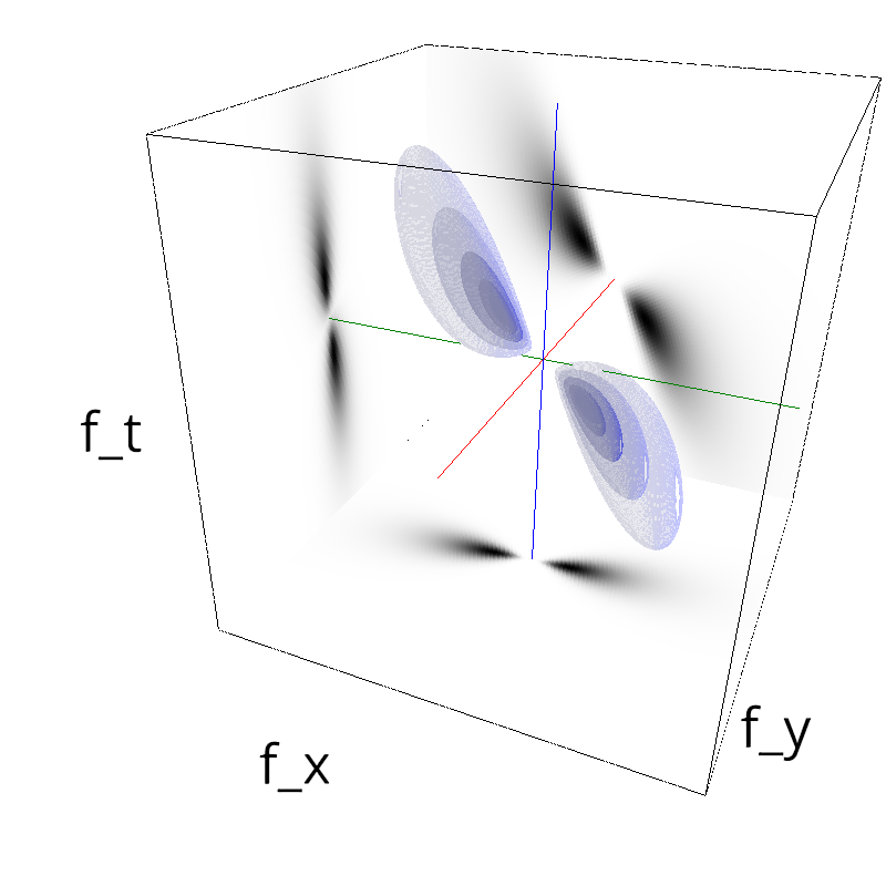
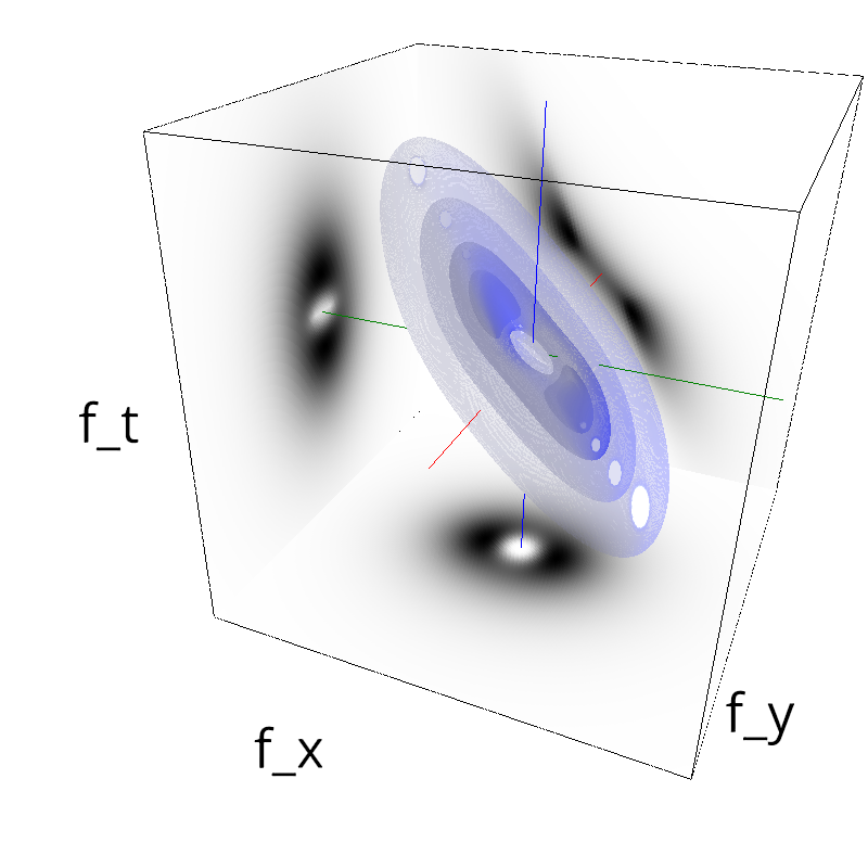
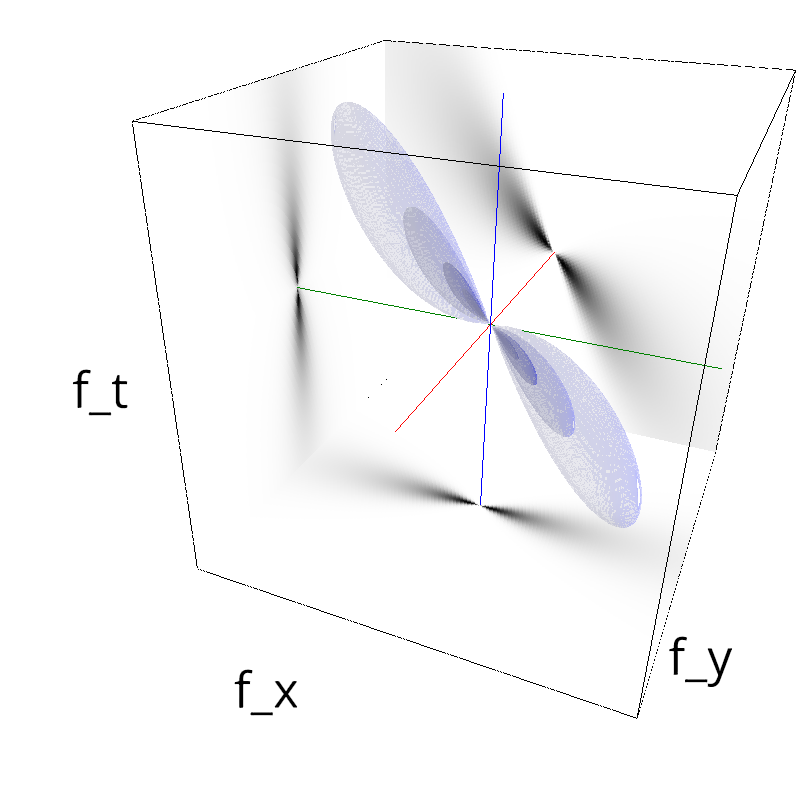
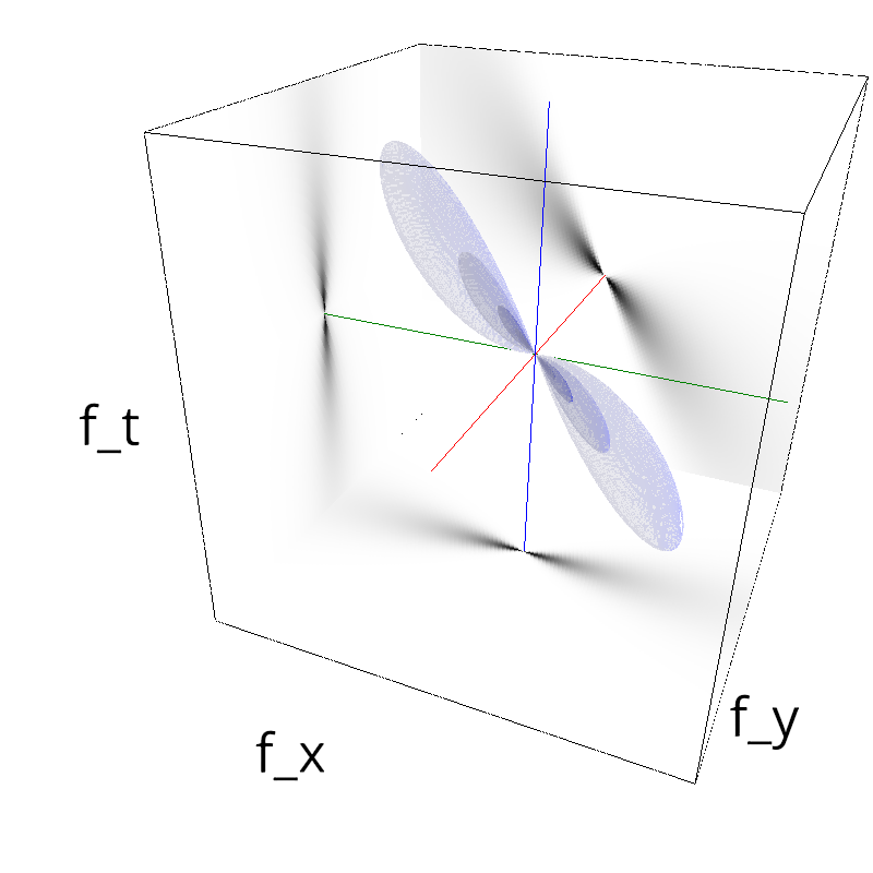
for div in [1, 2, 4, 3, 5, 8, 13, 20, 30]:
    name_ = name + '-theta-pi-over-' + str(div).replace('.', '_')
    z = mc.envelope_gabor(fx, fy, ft, theta=np.pi/div)
    mc.figures(z, name_)
    mc.in_show_video(name_)
 |
||
 |
||
 |
||
 |
||
 |
||
 |
||
 |
||
 |
||
 |
||
 |
||
 |
||
 |
||
 |
||
 |
||
 |
||
 |
||
 |
||
 |
||
V_X = 1.0
for sigma_div in [1, 2, 3, 5, 8, 13 ]:
    name_ = name + '-B_theta-pi-over-' + str(sigma_div).replace('.', '_') + '-V_X-' + str(V_X).replace('.', '_')
    z = mc.envelope_gabor(fx, fy, ft, V_X=V_X, B_theta=np.pi/sigma_div)
    mc.figures(z, name_)
    mc.in_show_video(name_)
 |
||
 |
||
 |
||
 |
||
 |
||
 |
||
 |
||
 |
||
 |
||
 |
||
 |
||
 |
||
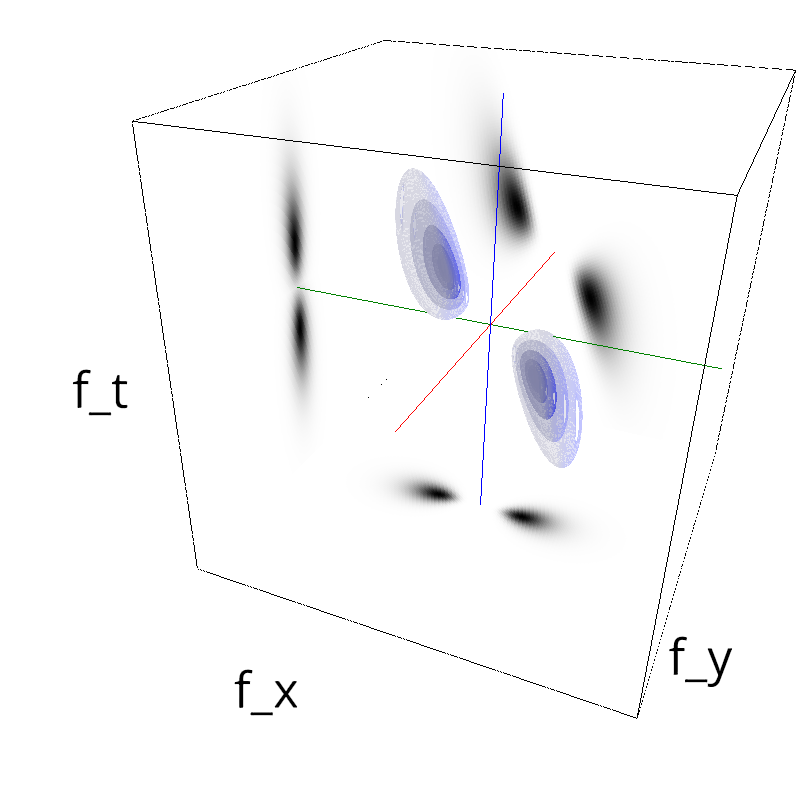
for B_sf in [0.05, 0.1, 0.15, 0.2, 0.3, 0.4, 0.8]:
    name_ = name + '-B_sf-' + str(B_sf).replace('.', '_')
    z = mc.envelope_gabor(fx, fy, ft, B_sf=B_sf)
    mc.figures(z, name_)
    mc.in_show_video(name_)
 |
||
 |
||
 |
||
 |
||
 |
||
 |
||
 |
||
 |
||
 |
||
 |
||
 |
||
 |
||
 |
||
 |
||
tuning the bandwidth
In the MotionClouds script, we define the orientation envelope based on a VonMises distribution:
def vonmises(th, theta, kappa, norm=True):
    if kappa==0:
        env = np.ones_like(th)
    elif kappa==np.inf:
        env = np.zeros_like(th)
        env[np.argmin(th < theta)] = 1.
    else:
        env = np.exp(kappa*(np.cos(2*(th-theta))-1))
    if norm:
        return env/env.sum()
    else:
        return env
This definition handles also the extreme cases when the bandwidth is infinite (in which case we return a flat distribution) of null (so we get a dirac). Note also that the von Mises distribution is on a continuous variable (orientation), while we use a discrete fourier transform. In particular, some care should be taken for very narrow bandwidths.
N_theta = 16
theta, B_sf, B_V = np.pi/2, .1, .3
bins = 60
th = np.linspace(0, np.pi, bins, endpoint=False)
fig, ax = plt.subplots(1, 1, figsize=(13, 8))
B_theta_ = [np.pi/640, np.pi/32, np.pi/16, np.pi/8, np.pi/4, np.pi/2, np.inf]
for B_theta, color in zip(B_theta_, [plt.cm.hsv(h) for h in np.linspace(0, 1, len(B_theta_))]):
    kappa = 1./4/B_theta**2
    ax.plot(th, vonmises(th, theta, kappa), alpha=.6, color=color, lw=3)
    ax.fill_between(th, 0, vonmises(th, theta, B_theta), alpha=.1, color=color)
    ax.set_xlabel('orientation (radians)')
_ = ax.set_xlim([0, np.pi])

Getting everything peaking at one:
N_theta = 16
theta, B_sf, B_V = np.pi/2, .1, .3
bins = 360
th = np.linspace(0, np.pi, bins, endpoint=False)
fig, ax = plt.subplots(1, 1, figsize=(13, 8))
for B_theta, color in zip(B_theta_, [plt.cm.hsv(h) for h in np.linspace(0, 1, len(B_theta_))]):
    kappa = 1./4/B_theta**2
    ax.plot(th, vonmises(th, theta, kappa, norm=False), alpha=.6, color=color, lw=3)
    ax.fill_between(th, 0, vonmises(th, theta, kappa, norm=False), alpha=.1, color=color)
    ax.set_xlabel('orientation (radians)')
_ = ax.set_xlim([0, np.pi])

Let's check that the HWHH (half-width at half-height) is given by the bandwidth parameter B_theta. Note that for high values of B_theta, the minimum of the distribution may be higher than 1/2 and that this decriptive value may be ill-defined (see for instance Swindale, N. V. (1998). Orientation tuning curves: empirical description and estimation of parameters. Biological Cybernetics, 78(1):45-56 - PDF). We will use the broader definition by using the fully normalized von mises that peaks at one and with a minimum at 0 :
$$M(\theta) = \frac {\exp( \kappa \cdot cos(2\theta)) - \exp( -\kappa) }{\exp(\kappa) - \exp( -\kappa) }$$
The different expression for the HWHH are for the Gaussian approximation:
$$\theta_{HWHH} = \sqrt{2\ln(2)} \cdot \kappa $$
for the non-normalized von-Mises pdf (as in Swindale):
$$\theta_{HWHH} = \frac 1 2 \cdot \arccos (1 + \frac{ \ln( \frac 1 2 )}{\kappa})$$for the normalized (exact) solution:
$$\theta_{HWHH} = \frac 1 2 \cdot \arccos (1 + \frac{\ln(\frac{1+e^{-2\kappa})}{2}}{\kappa})$$
N_theta = 160
theta, B_sf, B_V = 0, .1, .3
B_theta_ = np.linspace(0, np.pi/2, N_theta, endpoint=False)
bins = 3600
th = np.linspace(0, np.pi, bins, endpoint=False)
HWHH = np.zeros(N_theta)
for _, B_theta in enumerate(B_theta_):
    kappa = 1./4/B_theta**2
    dist = vonmises(th, theta, kappa)
    dist = (dist - dist.min())/(dist.max() - dist.min())
    ind_HWHH = np.argmax(dist<.5)
    HWHH[_] = th[ind_HWHH]

fig, ax = plt.subplots(1, 1, figsize=(13, 8))
ax.plot(B_theta_, HWHH, 'k+', label='observed')
ax.plot(B_theta_, B_theta_*np.sqrt(2*np.log(2)), 'r', label='gaussian')
k= 1./4/B_theta_**2
ax.plot(B_theta_, .5*np.arccos(1-np.log(2)/k), 'b', label='swindale')
ax.plot(B_theta_, .5*np.arccos(1+ np.log((1+np.exp(-2*k))/2)/k), 'g', label='exact')
ax.set_xlabel('B_theta (radians)')
ax.set_ylabel('HWHH (radians)')
ax.legend()
_ = ax.set_xlim([0, np.pi/2])

This shows that in the range of relevant values of B_theta (that is inferior to approximately 60 degrees) we can control the bandwidth as for a Gaussian or a von-Mises curve, while for higher values, the distribution can be considered to be flat.