Testing the utility functions of Motion Clouds
Motion Clouds utilities
Here, we test some of the utilities that are delivered with the MotionClouds package.
%load_ext autoreload
%autoreload 2
import os
import MotionClouds as mc
mc.N_X, mc.N_Y, mc.N_frame = 30, 40, 50
fx, fy, ft = mc.get_grids(mc.N_X, mc.N_Y, mc.N_frame)
generating figures
As they are visual stimuli, the main outcome of the scripts are figures. Utilities allow to plot all figures, usually marked by a name:
name = 'testing_utilities'
help(mc.figures_MC)
mc.figures_MC(fx, fy, ft, name, recompute=True)
help(mc.in_show_video)
mc.in_show_video(name)
 |
||
 |
||
This function embeds the images and video within the notebook. Sometimes you want to avoid that:
mc.in_show_video(name, embed=False)
|
||
|
||
Sometimes, you may have already computed some envelope or just want to distort it, then you can use mc.figures:
env = mc.envelope_gabor(fx, fy, ft)
help(mc.figures)
import numpy as np
mc.figures(np.sqrt(env), name + '_0')
mc.in_show_video(name + '_0')
 |
||
 |
||
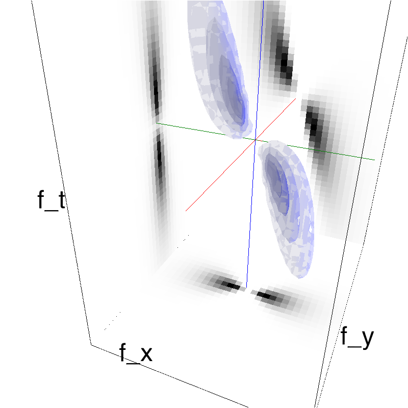
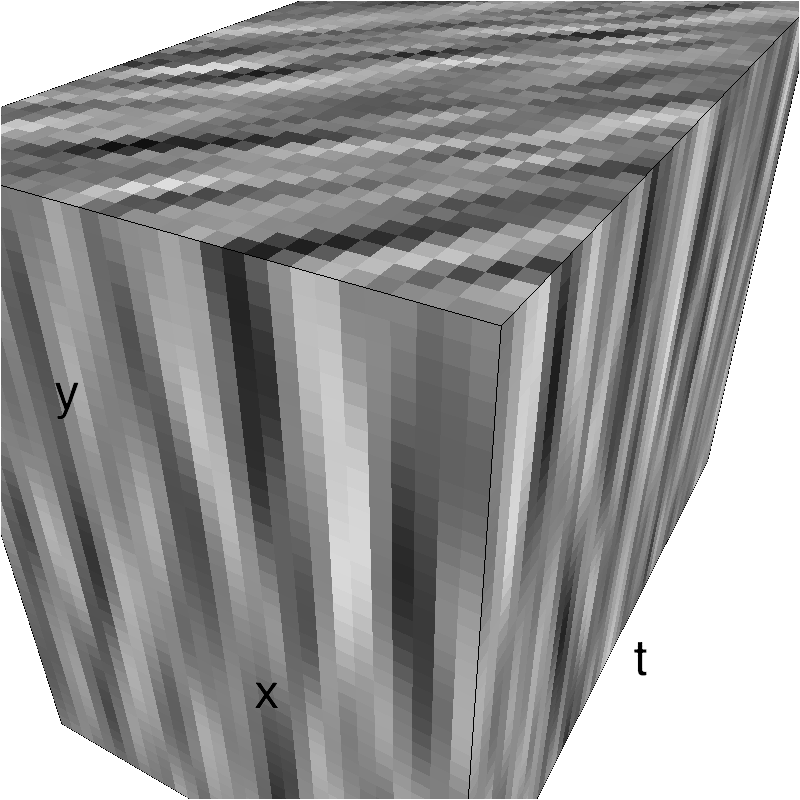
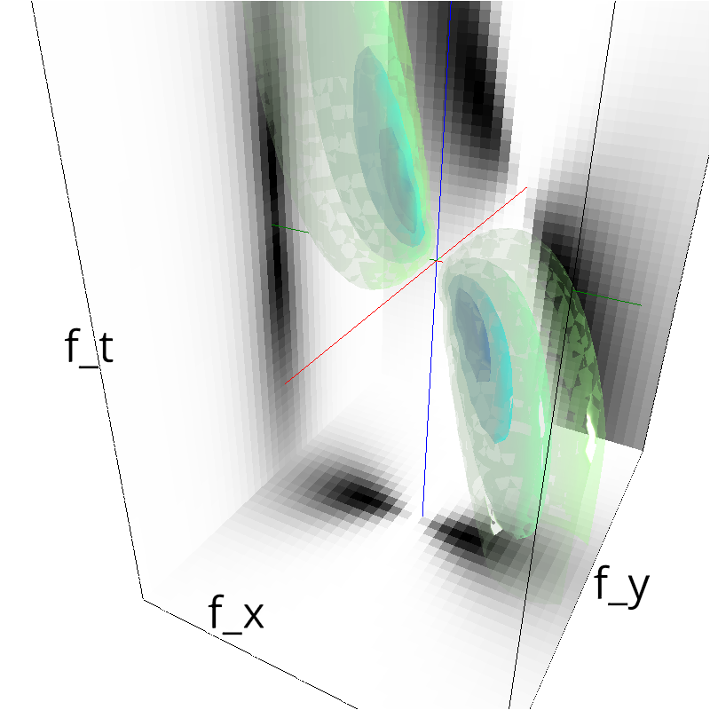
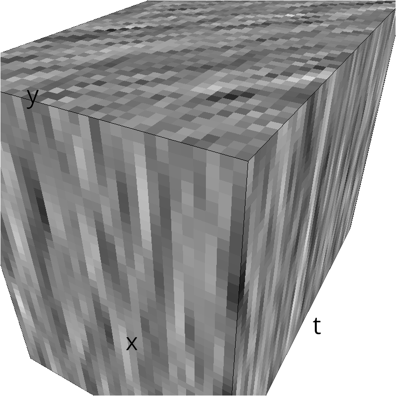
low-level figures : 3D visualizations
help(mc.cube)
help (mc.visualize)
Handling filenames
By default, the folder for generating figures or data is mc.figpath:
print(mc.figpath)
To generate figures, we assign file names, such as:
filename = os.path.join(mc.figpath, name)
It is then possible to check if that figures exist:
print('filename=', filename, ', exists? : ', mc.check_if_anim_exist(filename))
Note that the file won't be recomputed if it exists:
mc.figures(env, name)
This behavior can be overriden using the recompute option
mc.figures(env, name, recompute=True)
Warning: be sure that when you display a given file, it corresponds to the parameters you have set for your stimulus.
low-level figures : exporting to various formats
It is possible to export motion clouds to many different formats. Here are some examples:
!rm -fr ../files/export
name = 'export'
fx, fy, ft = mc.get_grids(mc.N_X, mc.N_Y, mc.N_frame)
z = mc.rectif(mc.random_cloud(mc.envelope_gabor(fx, fy, ft)))
mc.PROGRESS = False
for vext in mc.SUPPORTED_FORMATS:
    print ('Exporting to format: ', vext)
    mc.anim_save(z, os.path.join(mc.figpath, name), display=False, vext=vext, verbose=False)
showing a video
To show a video in a notebook, issue:
mc.notebook = True # True by default
mc.in_show_video('export')
Rectifying the contrast
The mc.rectif function allows to rectify the amplitude of luminance values within the whole generated texture between $0$ and $1$:
fx, fy, ft = mc.get_grids(mc.N_X, mc.N_Y, mc.N_frame)
envelope = mc.envelope_gabor(fx, fy, ft)
image = mc.random_cloud(envelope)
print('Min :', image.min(), ', mean: ', image.mean(), ', max: ', image.max())
image = mc.rectif(image)
print('Min :', image.min(), ', mean: ', image.mean(), ', max: ', image.max())
import pylab
import numpy as np
import matplotlib.pyplot as plt
import math
%matplotlib inline
#%config InlineBackend.figure_format='retina' # high-def PNGs, quite bad when using file versioning
%config InlineBackend.figure_format='svg'
name = 'contrast_methods-'
#initialize
fx, fy, ft = mc.get_grids(mc.N_X, mc.N_Y, mc.N_frame)
ext = '.zip'
contrast = 0.25
B_sf = 0.3

for method in ['Michelson', 'Energy']:
    z = mc.envelope_gabor(fx, fy, ft, B_sf=B_sf)
    im = np.ravel(mc.random_cloud(z, seed =1234))
    im_norm = mc.rectif(mc.random_cloud(z), contrast, method=method, verbose=True)
    plt.figure()
    plt.subplot(111)
    plt.title(method + ' Histogram Ctr: ' + str(contrast))
    plt.ylabel('pixel counts')
    plt.xlabel('grayscale')
    bins = int((np.max(im_norm[:])-np.min(im_norm[:])) * 256)
    plt.xlim([0, 1])
    plt.hist(np.ravel(im_norm), bins=bins, normed=False, facecolor='blue', alpha=0.75)
    #plt.savefig(name_)

def image_entropy(img):
    """calculate the entropy of an image"""
    histogram = img.histogram()
    histogram_length = np.sum(histogram)
    samples_probability = [float(h) / histogram_length for h in histogram]
    return -np.sum([p * math.log(p, 2) for p in samples_probability if p != 0])
If we normalise the histogram then the entropy base on gray levels is going to be the almost the same.
TODO: Review the idea of entropy between narrowband and broadband stimuli.