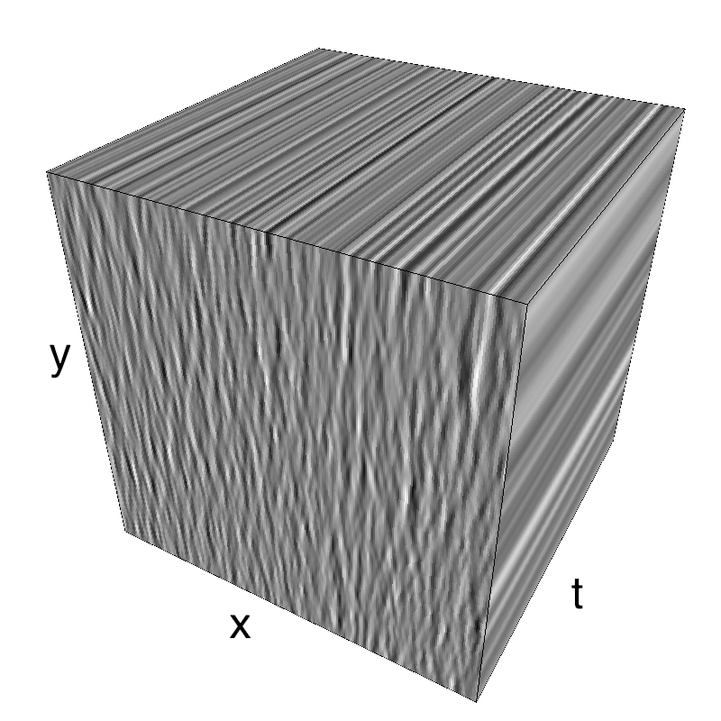
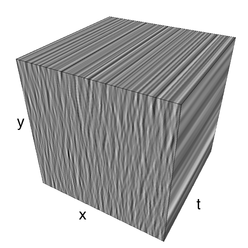
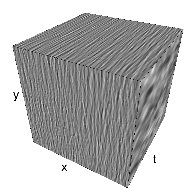
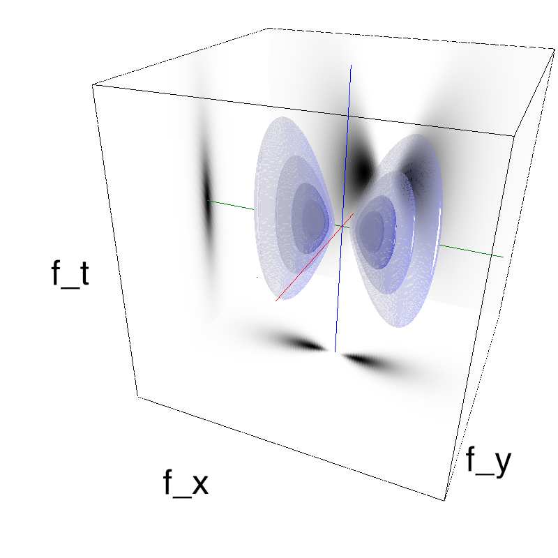
Returns the speed envelope:
selects the plane corresponding to the speed ``(V_X, V_Y)`` with some bandwidth ``B_V``.
* (V_X, V_Y) = (0,1) is downward and (V_X, V_Y) = (1, 0) is rightward in the movie.
* A speed of V_X=1 corresponds to an average displacement of 1/N_X per frame.
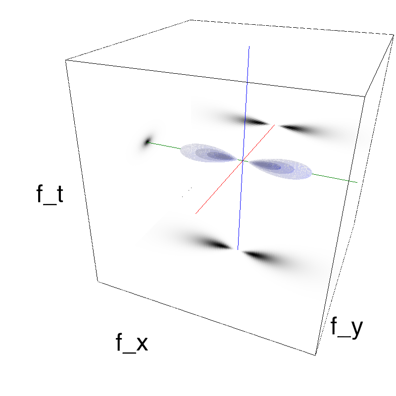
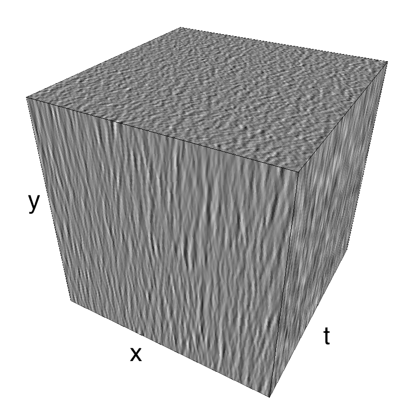
To achieve one spatial period in one temporal period, you should scale by
V_scale = N_X/float(N_frame)
If N_X=N_Y=N_frame and V=1, then it is one spatial period in one temporal
period. It can be seen along the diagonal in the fx-ft face of the MC cube.
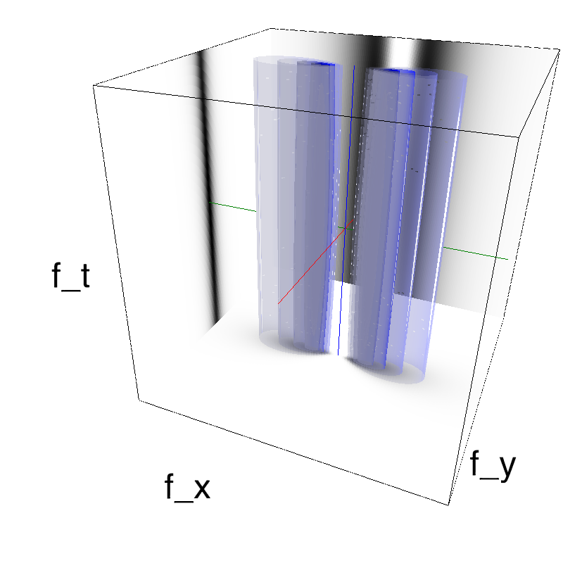
A special case is used when ``B_V=0``, where the ``fx-ft`` plane is used as
the speed plane: in that case it is desirable to set ``(V_X, V_Y)`` to ``(0, 0)``
to avoid aliasing problems.
Run the 'test_speed' notebook to explore the speed parameters, see
http://motionclouds.invibe.net/posts/testing-speed.html